
Matrix Factorization with Tensorflow
Mar 11, 2016 · 9 minute read · CommentsI’ve been working on building a content recommender in TensorFlow using matrix factorization, following the approach described in the article Matrix Factorization Techniques for Recommender Systems (MFTRS). I haven’t come across any discussion of this particular use case in TensorFlow but it seems like an ideal job for it. I’ll explain briefly here what matrix factorization is in the context of recommender systems (although I highly cough recommend reading the MFTRS article) and how things needed to be set up to do this in TensorFlow. Then I’ll show the code I wrote to train the model and the resulting TensorFlow computation graph produced by TensorBoard.
The basics
A matrix of ratings with users as rows and items as columns might look something like this:
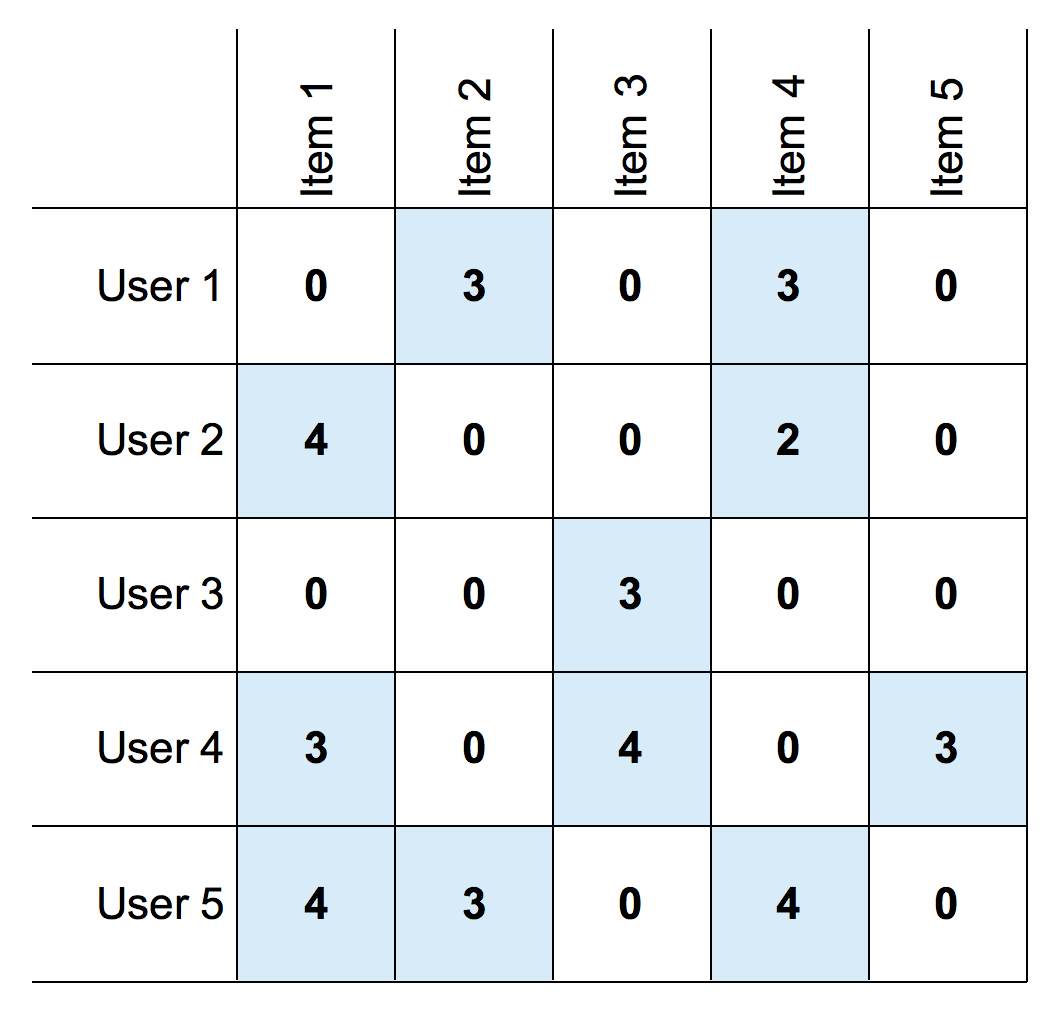
A matrix of user/item ratings
We see for example that user 1 has given item 2 a rating of 3.
What matrix factorization does is to come up with two smaller matrices, one representing users and one representing items, which when multiplied together will produce roughly this matrix of ratings, ignoring the 0 entries.
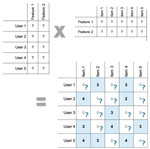
So if our original matrix is m x n, where m is the number of users and n is the number of items, we need an m x d matrix and a d x n matrix as our factors, where d is chosen to be small enough for the computation to be efficient and large enough to represent the number of dimensions along which interactions between users and items are likely to vary in some significant way. In the above illustration we have d = 2. The predicted rating by a given user for a given item is then the dot product of the vector representing the user and the vector representing the item. In the MFTRS article, this is expressed as:
$ \hat{r_{ui}} = q_i^Tp_u $
where $ \hat{r_{ui}} $ denotes the predicted rating for user u and item i and $ q_i^Tp_u $ denotes the dot product of the vector representing item i and the vector representing user u.
User bias, item bias and average rating
We need to add bias into the mix. Each user’s average rating will be different from the average rating across all users. And the average rating of a particular item will be somewhat different from the average across all items.
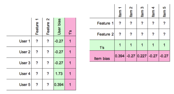
Adding user and item bias
Adding a column vector of user bias to the user matrix and matching it with a row vector of 1s in the item matrix has the effect that the rating prediction for a given user/item pair will now have that user’s bias added on. Similarly, adding a row vector of item biases to items and a matching column vector of 1s to users will add the item bias to the prediction.
The average rating across all users and items also needs to be included so in the notation of the MFTRS article each rating will be predicted using:
$ \hat{r_{ui}} = \mu + b_i + b_u + q_i^Tp_u $
where $ \mu $ is the overall average rating, $ b_i $ is the bias for item i, $ b_u $ is the bias for user u, and $ q_i^Tp_u $ is the interaction between item i and user u.
But the overall mean rating can be added on after we do the matrix multiplication.
Objective Function and Regularization
The objective function, or cost function, used in this approach is simply the sum of squared distances between predicted ratings and actual ratings, so this is what we need to minimize. But in order to prevent over-fitting to the training data we need to constrain the learned values for our user and item features by penalizing high values. We do this by multiplying the sum of the squares of the elements of the user and item matrices by a configurable regularization parameter and including this in our cost function. We’ll use gradient descent to minimize the cost.
Accuracy
The metric I decided on for accuracy was to calculate the fraction of predicted ratings that were within some threshold of the real rating. I used a threshold of 0.5 when evaluating accuracy. Note that this type of absolute threshold works fine if the ratings are on a fixed scale, e.g. 1-5, but for something like the Million Song Dataset, where “ratings” are actually listen counts, a percentage based threshold would need to be used.
Sparse representation of matrices
The ratings matrix is sparse, meaning most of the values are 0, because each user has only rated a small number of items. The concept of a sparse matrix can actually be translated to a different data structure that retains only information about the non-zero values, making it a much more memory-efficient represenation of the same information. One way is to define a vector of row indices, i, a vector of column indices, j, and a vector of values for each (i,j) pair. So only the (i,j) pairs that have values are included. Using this format, known as coordinate list or COO, the above ratings would be expressed as follows:
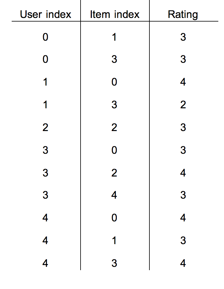
The same ratings in COO sparse matrix format
The dataset I worked with was the Movie Lens dataset, available here. Only the u.data file was needed to train the model. This contains 100,000 ratings from 943 users of 1,682 movies. If we expressed this as a full matrix, we’d have 943 x 1,682 = 1,586,126 values to store in memory while doing computations on them. But doing it this way we only have to work with 100,000 x 3 = 300,000 values.
The user_ids and item_ids in this dataset are already serial IDs, so we have users 1 through 943 and items 1 through 1682. Subracting 1 from each ID allows us to use them as matrix indices. They also need to be ordered first by user index, then by item index for faster access.
The Code
The code below assumes we have training ratings and validation ratings in the above COO format and have extracted the individual columns as the row_indices, col_indices and rating_values variables, in the case of the training set, and variables suffixed with _val for the validation set. For more complete example code, see the Beaker notebook here.
The configurable parameters are
- rank, or number of feature vectors to learn
- lamda (regularization parameter)
- learning rate
- accuracy threshold
# Initialize the matrix factors from random normals with mean 0. W will
# represent users and H will represent items.
W = tf.Variable(tf.truncated_normal([num_users, rank], stddev=0.2, mean=0), name="users")
H = tf.Variable(tf.truncated_normal([rank, num_items], stddev=0.2, mean=0), name="items")

# To the user matrix we add a bias column holding the bias of each user,
# and another column of 1s to multiply the item bias by.
W_plus_bias = tf.concat(1, [W, tf.convert_to_tensor(user_bias, dtype=float32, name="user_bias"), tf.ones((num_users,1), dtype=float32, name="item_bias_ones")])
# To the item matrix we add a row of 1s to multiply the user bias by, and
# a bias row holding the bias of each item.
H_plus_bias = tf.concat(0, [H, tf.ones((1, num_items), name="user_bias_ones", dtype=float32), tf.convert_to_tensor(item_bias, dtype=float32, name="item_bias")])
# Multiply the factors to get our result as a dense matrix
result = tf.matmul(W_plus_bias, H_plus_bias)

# Now we just want the values represented by the pairs of user and item
# indices for which we had known ratings. Unfortunately TensorFlow does not
# yet support numpy-like indexing of tensors. See the issue for this at
# https://github.com/tensorflow/tensorflow/issues/206 The workaround here
# came from https://github.com/tensorflow/tensorflow/issues/418 and is a
# little esoteric but in numpy this would just be done as follows:
# result_values = result[user_indices, item_indices]
result_values = tf.gather(tf.reshape(result, [-1]), user_indices * tf.shape(result)[1] + item_indices, name="extract_training_ratings")

# Same thing for the validation set ratings.
result_values_val = tf.gather(tf.reshape(result, [-1]), user_indices_val * tf.shape(result)[1] + item_indices_val, name="extract_validation_ratings")

# Calculate the difference between the predicted ratings and the actual
# ratings. The predicted ratings are the values obtained form the matrix
# multiplication with the mean rating added on.
diff_op = tf.sub(tf.add(result_values, mean_rating, name="add_mean"), rating_values, name="raw_training_error")
diff_op_val = tf.sub(tf.add(result_values_val, mean_rating, name="add_mean_val"), rating_values_val, name="raw_validation_error")

with tf.name_scope("training_cost") as scope:
    base_cost = tf.reduce_sum(tf.square(diff_op, name="squared_difference"), name="sum_squared_error")
    # Add regularization.
    regularizer = tf.mul(tf.add(tf.reduce_sum(tf.square(W)), tf.reduce_sum(tf.square(H))), lda, name="regularize")
    cost = tf.div(tf.add(base_cost, regularizer), num_ratings * 2, name="average_error")

with tf.name_scope("validation_cost") as scope:
    cost_val = tf.div(tf.reduce_sum(tf.square(diff_op_val, name="squared_difference_val"), name="sum_squared_error_val"), num_ratings_val * 2, name="average_error")

# Use an exponentially decaying learning rate.
global_step = tf.Variable(0, trainable=False)
learning_rate = tf.train.exponential_decay(lr, global_step, 10000, 0.96, staircase=True)


with tf.name_scope("train") as scope:
    optimizer = tf.train.GradientDescentOptimizer(learning_rate)
    # Passing global_step to minimize() will increment it at each step so
    # that the learning rate will be decayed at the specified intervals.
    train_step = optimizer.minimize(cost, global_step=global_step)

with tf.name_scope("training_accuracy") as scope:
  # Just measure the absolute difference against the threshold
  # TODO: support percentage-based thresholds
  good = tf.less(tf.abs(diff_op), threshold)

  accuracy_tr = tf.div(tf.reduce_sum(tf.cast(good, tf.float32)), num_ratings)
  accuracy_tr_summary = tf.scalar_summary("accuracy_tr", accuracy_tr)

with tf.name_scope("validation_accuracy") as scope:
  # Validation set accuracy:
  good_val = tf.less(tf.abs(diff_op_val), threshold)
  accuracy_val = tf.reduce_sum(tf.cast(good_val, tf.float32)) / num_ratings_val
  accuracy_val_summary = tf.scalar_summary("accuracy_val", accuracy_val)

# Create a TensorFlow session and initialize variables.
sess = tf.Session()
sess.run(tf.initialize_all_variables())

# Make sure summaries get written to the logs.
summary_op = tf.merge_all_summaries()
writer = tf.train.SummaryWriter("/tmp/recommender_logs", sess.graph_def)

# Run the graph and see how we're doing on every 500th iteration.
for i in range(max_iter):
    if i % 500 == 0:
        res = sess.run([summary_op, accuracy_tr, accuracy_val, cost, cost_val])
        summary_str = res[0]
        acc_tr = res[1]
        acc_val = res[2]
        cost_ev = res[3]
        cost_val_ev = res[4]
        writer.add_summary(summary_str, i)
        print("Training accuracy at step %s: %s" % (i, acc_tr))
        print("Validation accuracy at step %s: %s" % (i, acc_val))
        print("Training cost: %s" % (cost_ev))
        print("Validation cost: %s" % (cost_val_ev))
    else:
        sess.run(train_step)

with tf.name_scope("final_model") as scope:
    # At the end we want to get the final ratings matrix by adding the mean
    # to the result matrix and doing any further processing required
    add_mean_final = tf.add(result, mean_rating, name="add_mean_final")
    if result_processor == None:
        final_matrix = add_mean_final
    else:
        final_matrix = result_processor(add_mean_final)
    final_res = sess.run([final_matrix])
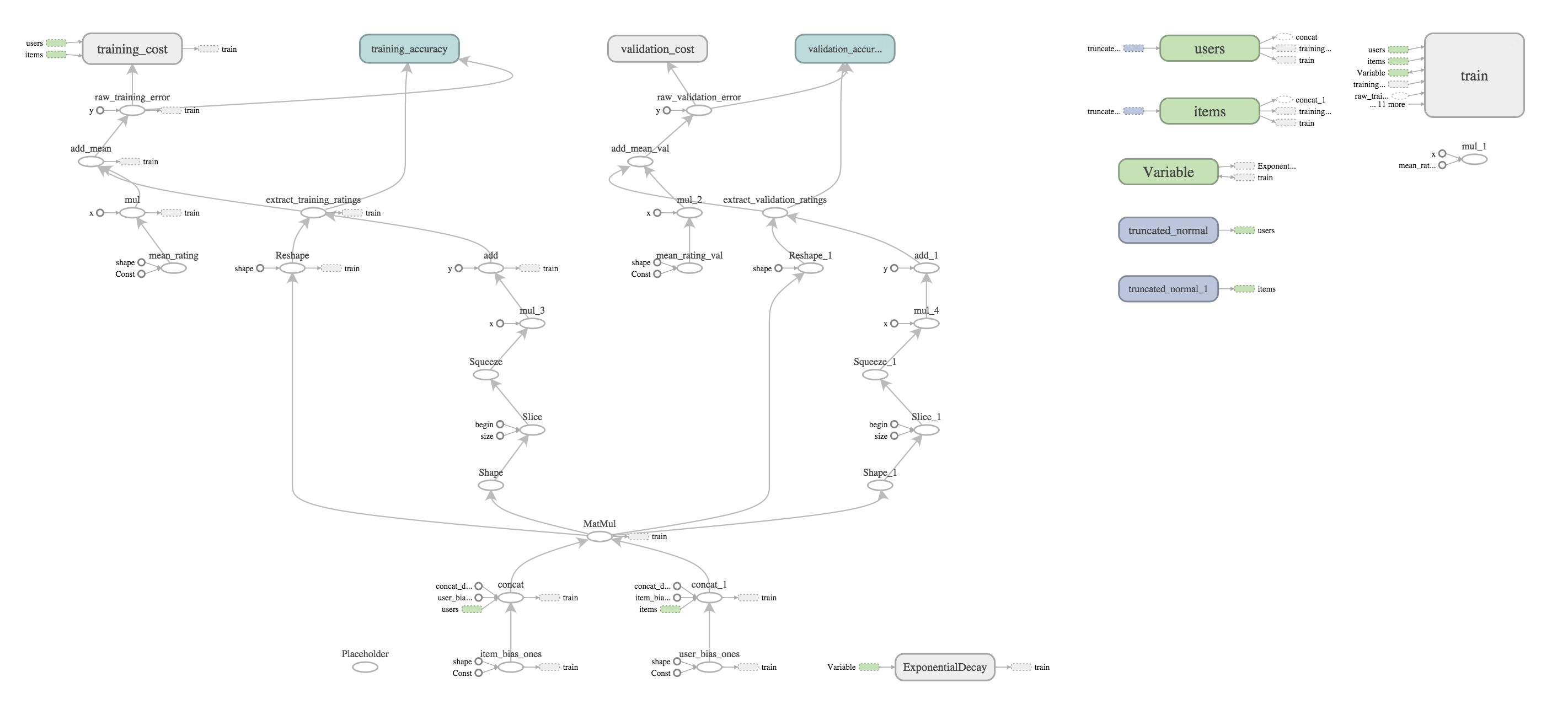
Computation Graph
Here is the overall computation graph produced by this code as visualized by TensorBoard. Click the image to enlarge it.
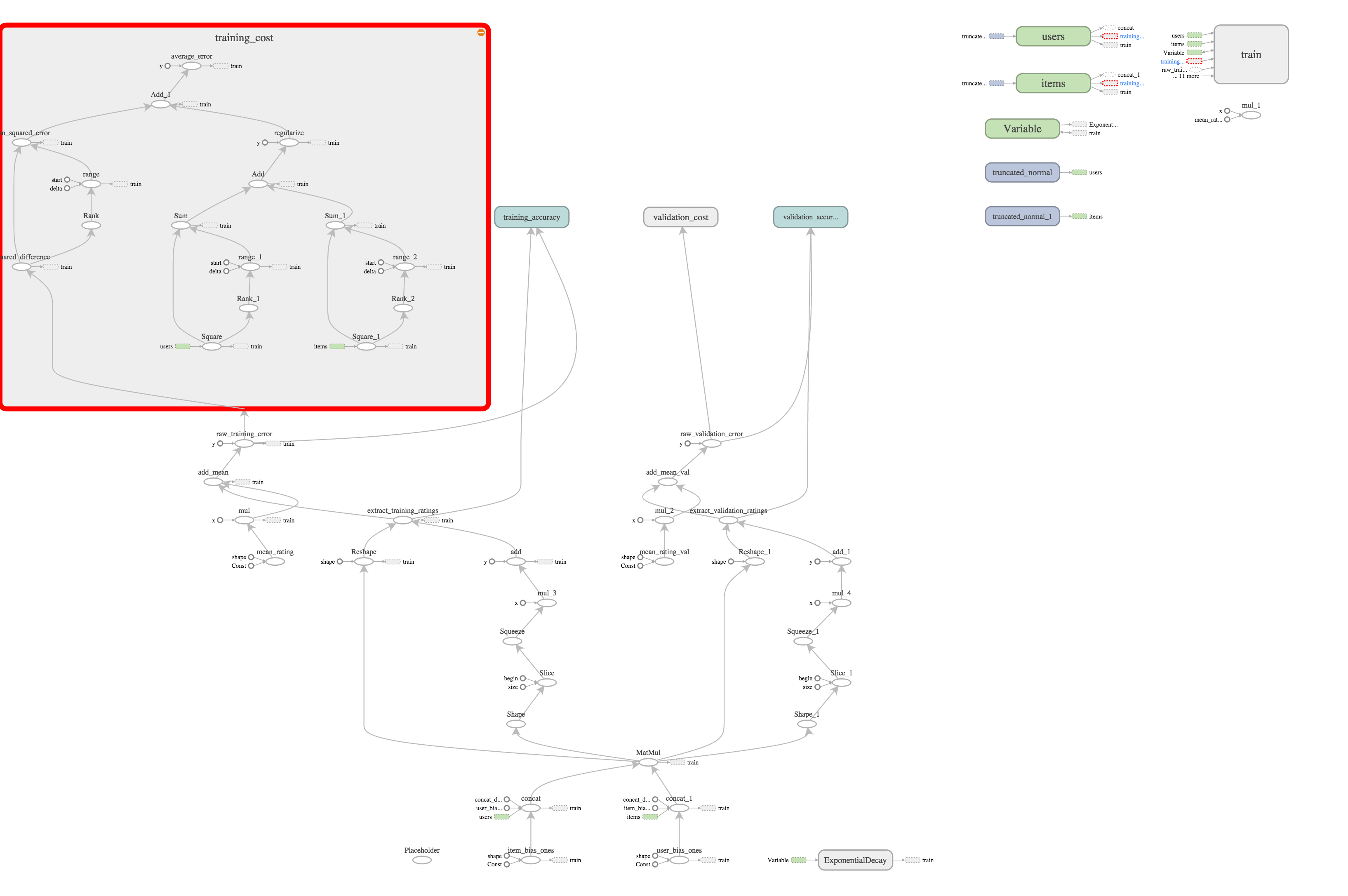
And here’s the training cost portion of the graph expanded.
Results and Next Steps
OK, this is the part where I come clean and admit that I have not yet spent sufficient time tweaking all the tweakable things to train a model that performs satisfactorily on unseen data. Very disappointingly, I haven’t seen better than 42% accuracy on the validation set. With an accuracy threshold of 0.5, this means that only roughly two out of five predicted ratings were within 0.5 of the actual rating. Not very impressive :(.
Interestingly though, the one time I ran it for 1 million iterations, the training accuracy never went above 60% and there had been no change in cost over the last several thousand iterations. This suggests that it got stuck in a local minimum and couldn’t get out.
I just started reading this paper on Probabilistic Matrix Factorization, which says in its introduction:
Since most real-world datasets are sparse, most entries in R will be missing. In those cases, the sum-squared distance is computed only for the observed entries of the target matrix R. As shown by (…), this seemingly minor modification results in a difficult non-convex optimization problem which cannot be solved using standard SVD implementations.
So my suspicion is that I have been taking a very naive approach to a highly non-convex optimization problem that no amount of parameter tuning is going to get me past. My next step will be to try to follow the probabilistic approach described in the above paper and present my findings in a follow-up post.