
Adventures learning Neural Nets and Python
Dec 21, 2015 · 18 minute read · CommentsThis documents my efforts to learn both neural networks and, to a certain extent, the Python programming language. I say “to a certain extent” because far from feeling all “yay! I know Python now!” I feel more like “I can use Python 2.7 in certain ways to do certain things… yay?”
And what of my understanding of neural nets as a result of this exercise? After battling with my naïve implementation of a multi-layer perceptron as described below, I felt I had a pretty visceral understanding of them. But then I started looking at Theano and Google’s TensorFlow with their convolutional neural networks etc, and it was the same old story: the more I learned, the more I realized I had yet to learn. So now there are all sorts of books and posts about various aspects of deep learning that I want to read, which I link to at this end of this post.
For a basic intro to how neural nets work, I recommend Sebastian Raschka’s post on Single-Layer Neural Networks. In short, though, the setup of a neural net for doing multi-class classification is as follows: at a minimum you have an input layer and an output layer. The input layer is the set of features you feed in and the output layer is the classification for each example. But you will likely also have at least one hidden layer as well.

A set of weights is applied to one layer to get to the next, until you reach the output layer, and training a neural network is about learning what these weights should be.
A little background
I recently took Andrew Ng’s Coursera course on Machine Learning. It’s taught through matlab and goes into the math behind classic machine learning algorithms such as neural networks. But I’ve been noticing that a lot of the newer code and tutorials out there for learning neural nets (e.g. Google’s TensorFlow tutorial) are in Python. So I thought, wouldn’t it be a fun exercise to port my matlab neural net to python and then learn about all the new libraries there are in python for doing this stuff, one of which is called Lasagne. Because layers :)
Here I use the handwritten digits dataset from the ML course assignment, which can be found here. It is much smaller than the MNIST dataset used in most tutorials, both in number of examples and in image size - each image is 20x20 pixels. I train 3 different neural networks:
- A simple port to Python of the matlab code I wrote for the ML course assignment
- An adaptation of the multi-layer perceptron from the Theano + Lasagne tutorial
- An adaptation of the convolutional neural net from the TensorFlow tutorial
Note: This is not a tutorial. It is simply an exploration, by a non-expert, of the topic of training neural nets in python. There are lots of great tutorials on this stuff, e.g. the ones mentioned below for Lasagne and TensorFlow, and also this one.
Initial Setup
Load some required libraries, extract the data from the matlab file and split it into training, validation and test sets.
from __future__ import print_function
import numpy as np
import scipy.io as sio
from sklearn.cross_validation import train_test_split
from pylab import *

mat_contents = sio.loadmat('ex4data1.mat')
# 0s were converted to 10s in the matlab data because matlab
# indices start at 1, so we need to change them back to 0s
labels = mat_contents['y']
labels = np.where(labels == 10, 0, labels)
labels = labels.reshape((labels.shape[0],))
X_train, X_test, y_train, y_test = train_test_split(mat_contents['X'], labels)
X_train, X_val = X_train[:-1000], X_train[-1000:]
y_train, y_val = y_train[:-1000], y_train[-1000:]
Here’s a visualization of one of the example images:
plt.imshow(X_train[1202].reshape((20, 20), order='F'), cmap='Greys', interpolation='nearest')
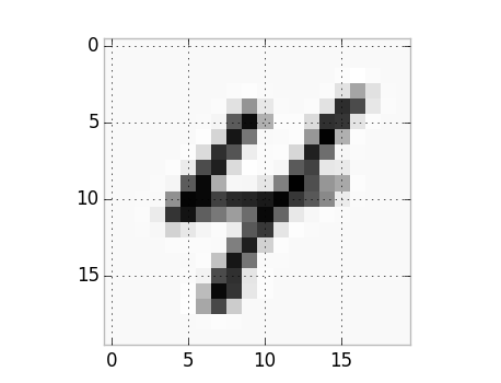
A number four from the training examples
1. Naïve neural net
This is where I just port the code I wrote in Matlab for the Coursera Machine Learning course into python. And where I learned that multiplying large matrices in Python is to be avoided :) More on that below, first here’s the code:
from scipy.optimize import minimize

# Basic sigmoid function for logistic regression.
def sigmoid(X):
    return 1.0 / (1.0 + math.e ** (-1.0 * X))

# Randomly initializes the weights for layer with the specified numbers of
# incoming and outgoing connections.
def randInitializeWeights(incoming, outgoing):
    epsilon_init = 0.12
    return rand(outgoing, 1 + incoming) * (2 * epsilon_init) - epsilon_init

# Adds the bias column to the matrix X.
def addBias(X):
    return np.concatenate((np.ones((X.shape[0],1)), X), 1)

# Reconstitutes the two weight matrices from a single vector, given the
# size of the input layer, the hidden layer, and the number of possible
# labels in the output.
def extractWeightMatrices(thetas, input_layer_size, hidden_layer_size, num_labels):
    theta1size = (input_layer_size + 1) * hidden_layer_size
    theta1 = reshape(thetas[:theta1size], (hidden_layer_size, input_layer_size + 1), order='A')
    theta2 = reshape(thetas[theta1size:], (num_labels, hidden_layer_size + 1), order='A')
    return theta1, theta2

# Converts single lables to one-hot vectors.
def convertLabelsToClassVectors(labels, num_classes):
    labels = labels.reshape((labels.shape[0],1))
    ycols = np.tile(labels, (1, num_classes))
    m, n = ycols.shape
    indices = np.tile(np.arange(num_classes).reshape((1,num_classes)), (m, 1))
    ymat = indices == ycols
    return ymat.astype(int)

# Returns a vector corresponding to the randomly initialized weights for the
# input layer and hidden layer.
def getInitialWeights(input_layer_size, hidden_layer_size, num_labels):
    theta1 = randInitializeWeights(input_layer_size, hidden_layer_size)
    theta2 = randInitializeWeights(hidden_layer_size, num_labels)
    return np.append(theta1.ravel(order='A'), theta2.ravel(order='A'))

# Trains a basic multilayer perceptron. Returns weights to use for feed-forward
# pass to predict on new data.
def train(X_train, y_train, hidden_layer_size, lmda, maxIter):
    input_layer_size = X_train.shape[1]
    num_labels = 10
    initial_weights = getInitialWeights(input_layer_size, hidden_layer_size, num_labels)
    if y_train.ndim == 1:
        # Convert the labels to one-hot vectors.
        y_train = convertLabelsToClassVectors(y_train, num_labels)

    # Given weights for the input layer and hidden layer, calulates the
    # activations for the hidden layer and the output layer of a 3-layer nn.
    def getActivations(theta1, theta2):
        z2 = np.dot(addBias(X_train),theta1.T)
        a2 = np.concatenate((np.ones((z2.shape[0],1)), sigmoid(z2)), 1)
        # a2 is an m x num_hidden+1 matrix, Theta2 is a num_labels x
        # num_hidden+1 matrix
        z3 = np.dot(a2,theta2.T)
        a3 = sigmoid(z3) # Now we have an m x num_labels matrix
        return a2, a3

    # Cost function to be minimized with respect to weights.
    def costFunction(weights):
        theta1, theta2 = extractWeightMatrices(weights, input_layer_size, hidden_layer_size, num_labels)
        hidden_activation, output_activation = getActivations(theta1, theta2)
        m = X_train.shape[0]
        cost = sum((-y_train * log(output_activation)) - ((1 - y_train) * log(1-output_activation))) / m
        # Regularization
        thetasq = sum(theta1[:,1:(input_layer_size + 1)]**2) + sum(theta2[:,1:hidden_layer_size + 1]**2)
        reg = (lmda / float(2*m)) * thetasq
        print("Training loss:\t\t{:.6f}".format(cost))
        return cost + reg

    # Gradient function to pass to our optimization function.
    def calculateGradient(weights):
        theta1, theta2 = extractWeightMatrices(weights, input_layer_size, hidden_layer_size, num_labels)
        # Backpropagation - step 1: feed-forward.
        hidden_activation, output_activation = getActivations(theta1, theta2)
        m = X_train.shape[0]
        # Step 2 - the error in the output layer is just the difference
        # between the output layer and y
        delta_3 = output_activation - y_train # delta_3 is m x num_labels
        delta_3 = delta_3.T

        # Step 3
        sigmoidGrad = hidden_activation * (1 - hidden_activation)
        delta_2 = (np.dot(theta2.T,delta_3)) * sigmoidGrad.T
        delta_2 = delta_2[1:, :] # hidden_layer_size x m
        theta1_grad = np.dot(delta_2, np.concatenate((np.ones((X_train.shape[0],1)), X_train), 1))
        theta2_grad = np.dot(delta_3, hidden_activation)
        # Add regularization
        reg_grad1 = (lmda / float(m)) * theta1
        # We don't regularize the weight for the bias column
        reg_grad1[:,0] = 0
        reg_grad2 = (lmda / float(m)) * theta2;
        reg_grad2[:,0] = 0
        return np.append(ravel((theta1_grad / float(m)) + reg_grad1, order='A'), ravel((theta2_grad / float(m)) + reg_grad2, order='A'))

    # Use scipy's minimize function with method "BFGS" to find the optimum
    # weights.
    res = minimize(costFunction, initial_weights, method='BFGS', jac=calculateGradient, options={'disp': False, 'maxiter':maxIter})
    theta1, theta2 = extractWeightMatrices(res.x, input_layer_size, hidden_layer_size, num_labels)
    return theta1, theta2

# Predicts the output given input and weights.
def predict(X, theta1, theta2):
    m, n = X.shape
    X = addBias(X)
    h1 = sigmoid(np.dot(X,theta1.T))
    h2 = sigmoid(addBias(h1).dot(theta2.T))
    return np.argmax(h2, axis=1)
That last function, predict, allows us to pass in a set of image representations, and some weights for the input and hidden layers, and it will predict the classification, i.e. which of digits 0 through 9 is represented by the image. First let’s see what we get with a random set of weights for each layer:
init_weights = getInitialWeights(400, 25, 10)
theta1_init, theta2_init = extractWeightMatrices(init_weights, 400, 25, 10)
pred_train = predict(X_train, theta1_init, theta2_init)
sum(np.where(y_train == pred_train, 1, 0))/float(X_train.shape[0])
0.11054545454545454
So, just over 11% accuracy, which when you think about it is roughly what you’d expect: given there are 10 possible classes for each image (digits 0 through 9), you have a 10% chance of getting it right simply by guessing.
So now let’s learn some better weights…
theta1, theta2 = nn.train(X_train, y_train, 25, 0, 50)
On my machine it takes about an hour to run this for 50 iterations. As an aside, I also tried to use it on the MNIST dataset. That dataset has 60,000 images of size 28x28 pixels. So the input layer consists of 784 features. With a hidden layer of 30 units it would grind away for a long time and eventually run out of memory. I managed to get it to run if I halved the number of hidden units.
I did some profiling using the awesome line_profiler to try to ascertain what the problem was. This helped me identify a few places where my code could be made more efficient - for example, initially I still had a for loop in the cost function - gasp! The first thing you learn in neural net school is the importance of using vectorized approaches to the computations. Anyway after I had fixed a few things like that it soon became clear to me that things weren’t getting hung inside any of my functions but in the optimization function itself. To cut a long story short, it was having to do a matrix multiplication where the matrices were 23860x23860. This number comes from the “unrolled” and concatenated weight vectors (with bias added on): (785 * 30) + (31*10). I have 16GB of RAM on my local machine, but that is apparently not enough for this operation to be run in Python. Both Theano and TensorFlow do all the heavy lifting in C, and this makes an enormous difference, as we’ll see.
Results after 50 iterations and no regularization
Training set:
predictions = predict(X_train, theta1, theta2)
sum(np.where(y_train == predictions, 1, 0))/float(X_train.shape[0])
Accuracy: 0.94145454545454543
Validation set:
predictions = predict(X_val, theta1, theta2)
sum(np.where(y_val == predictions, 1, 0))/float(X_val.shape[0])
Accuracy: 0.91900000000000004
Test set:
predictions = predict(X_test, theta1, theta2)
sum(np.where(y_test == predictions, 1, 0))/float(X_test.shape[0])
Accuracy: 0.91359999999999997
Not bad for just 50 iterations!
2. Using Theano and Lasagne
This code is adapted from the Lasagne tutorial (specifically the multi-layer perceptron.) I turned it into a function that works on the smaller data set and includes parameters for specifying:
- the number of units in its single hidden layer
- the number of epochs to run for
- the value to use for l2 regularization
- whether or not to use dropout layers (though the actual dropout probabilities for the input and hidden layers are hard-coded)
import time
import theano
import theano.tensor as T
import lasagne
from lasagne.regularization import regularize_layer_params_weighted, l2, l1

# Uses Lasagne to train a multi-layer perceptron, adapted from
# http://lasagne.readthedocs.org/en/latest/user/tutorial.html
def lasagne_mlp(X_train, y_train, X_val, y_val, X_test, y_test, hidden_units=25, num_epochs=500, l2_param = 0.01, use_dropout=True):
    X_train = X_train.reshape(-1, 1, 400)
    X_val = X_val.reshape(-1, 1, 400)
    X_test = X_test.reshape(-1, 1, 400)
    # Prepare Theano variables for inputs and targets
    input_var = T.tensor3('inputs')
    target_var = T.ivector('targets')

    print("Building model and compiling functions...")
    # Input layer
    network = lasagne.layers.InputLayer(shape=(None, 1, 400),
                                     input_var=input_var)

    if use_dropout:
        # Apply 20% dropout to the input data:
        network = lasagne.layers.DropoutLayer(network, p=0.2)

    # A single hidden layer with number of hidden units as specified in the
    # parameter.
    l_hid1 = lasagne.layers.DenseLayer(
            network, num_units=hidden_units,
            nonlinearity=lasagne.nonlinearities.rectify,
            W=lasagne.init.GlorotUniform())

    if use_dropout:
        # Dropout of 50%:
        l_hid1_drop = lasagne.layers.DropoutLayer(l_hid1, p=0.5)
        # Fully-connected output layer of 10 softmax units:
        network = lasagne.layers.DenseLayer(
            l_hid1_drop, num_units=10,
            nonlinearity=lasagne.nonlinearities.softmax)
    else:
        # Fully-connected output layer of 10 softmax units:
        network = lasagne.layers.DenseLayer(
            l_hid1, num_units=10,
            nonlinearity=lasagne.nonlinearities.softmax)

    # Loss expression for training
    prediction = lasagne.layers.get_output(network)
    loss = lasagne.objectives.categorical_crossentropy(prediction, target_var)
    loss = loss.mean()
    # Regularization.
    l2_penalty = lasagne.regularization.regularize_layer_params_weighted({l_hid1: l2_param}, l2)
    loss = loss + l2_penalty
    # Update expressions for training, using Stochastic Gradient Descent.
    params = lasagne.layers.get_all_params(network, trainable=True)
    updates = lasagne.updates.nesterov_momentum(
            loss, params, learning_rate=0.01, momentum=0.9)

    # Loss expression for evaluation.
    test_prediction = lasagne.layers.get_output(network, deterministic=True)
    test_loss = lasagne.objectives.categorical_crossentropy(test_prediction,
                                                            target_var)
    test_loss = test_loss.mean()
    # Expression for the classification accuracy:
    test_acc = T.mean(T.eq(T.argmax(test_prediction, axis=1), target_var),
                      dtype=theano.config.floatX)

    # Compile a function performing a training step on a mini-batch (by giving
    # the updates dictionary) and returning the corresponding training loss:
    train_fn = theano.function([input_var, target_var], loss, updates=updates)

    # Compile a second function computing the validation loss and accuracy:
    val_fn = theano.function([input_var, target_var], [test_loss, test_acc])

    # Finally, launch the training loop.
    print("Starting training...")
    # Keep track of taining and validation cost over the epochs
    epoch_cost_train = np.empty(num_epochs, dtype=float32)
    epoch_cost_val = np.empty(num_epochs, dtype=float32)
    # We iterate over epochs:
    for epoch in range(num_epochs):
        # In each epoch, we do a full pass over the training data:
        train_err = 0
        # We also want to keep track of the deterministic (feed-forward)
        # training error.
        train_err_ff = 0
        train_batches = 0
        start_time = time.time()
        for batch in iterate_minibatches(X_train, y_train, 50, shuffle=True):
            inputs, targets = batch
            err, acc = val_fn(inputs, targets)
            train_err_ff += err
            train_err += train_fn(inputs, targets)

            train_batches += 1

        # And a full pass over the validation data:
        val_err = 0
        val_acc = 0
        val_batches = 0
        for batch in iterate_minibatches(X_val, y_val, 50, shuffle=False):
            inputs, targets = batch
            err, acc = val_fn(inputs, targets)
            val_err += err
            val_acc += acc
            val_batches += 1

        epoch_cost_train[epoch] = train_err_ff / train_batches
        epoch_cost_val[epoch] = val_err / val_batches
        # Then we print the results for this epoch:
        print("Epoch {} of {} took {:.3f}s".format(
            epoch + 1, num_epochs, time.time() - start_time))
        print("  training loss:\t\t{:.6f}".format(train_err / train_batches))
        print("  validation loss:\t\t{:.6f}".format(val_err / val_batches))
        print("  validation accuracy:\t\t{:.2f} %".format(
            val_acc / val_batches * 100))

    # After training, we compute and print the test error:
    test_err = 0
    test_acc = 0
    test_batches = 0
    for batch in iterate_minibatches(X_test, y_test, 50, shuffle=False):
        inputs, targets = batch
        err, acc = val_fn(inputs, targets)
        test_err += err
        test_acc += acc
        test_batches += 1
    print("Final results:")
    print("  test loss:\t\t\t{:.6f}".format(test_err / test_batches))
    print("  test accuracy:\t\t{:.2f} %".format(
        test_acc / test_batches * 100))
    return epoch_cost_train, epoch_cost_val

# This function was copied verbatim from the Lasagne tutorial at
# http://lasagne.readthedocs.org/en/latest/user/tutorial.html
def iterate_minibatches(inputs, targets, batchsize, shuffle=False):
    assert len(inputs) == len(targets)
    if shuffle:
        indices = np.arange(len(inputs))
        np.random.shuffle(indices)
    for start_idx in range(0, len(inputs) - batchsize + 1, batchsize):
        if shuffle:
            excerpt = indices[start_idx:start_idx + batchsize]
        else:
            excerpt = slice(start_idx, start_idx + batchsize)
        yield inputs[excerpt], targets[excerpt]
Here we run it for 500 epochs without regularization but with dropout on the input and hidden layers.
epoch_cost_train, epoch_cost_val = lasagne_mlp(X_train, y_train, X_val, y_val, X_test,
 y_test, hidden_units=800, num_epochs=500, l2_param=0, use_dropout=True)
Epoch 1 of 500 took 0.495s
  training loss:                0.282050
  validation loss:              0.216164
  validation accuracy:          94.50 %
...
Epoch 500 of 500 took 0.504s
  training loss:                0.016550
  validation loss:              0.127085
  validation accuracy:          97.50 %
Final results:
  test loss:                    0.152830
  test accuracy:                96.48 %
Each epoch generally took less than a second to run. But one time I ran it and noticed it taking forever to run a single epoch - it would grind away and eventually get through one epoch after about 8 minutes. So I thought to myself “I wonder if that warning I saw but ignored when Theano got imported was actually important”… Yep. The warning was “WARNING (theano.configdefaults): g++ not detected ! Theano will be unable to execute optimized C-implementations (for both CPU and GPU) and will default to Python implementations. Performance will be severely degraded.” It couldn’t find g++ and so it was actually doing everything in Python. Turned out it was because I had upgraded XCode the previous day but the upgrade hadn’t completed (because I hadn’t opened it and accepted the license agreement). Anyway, the point here is: less than a second versus 8 minutes… holy shit!
Epoch 1 of 500 took 509.737s
  training loss:                1.544798
  validation loss:              0.795227
  validation accuracy:          83.20 %
Epoch 2 of 500 took 489.701s
  training loss:                0.730792
  validation loss:              0.512750
  validation accuracy:          86.90 %
Epoch 3 of 500 took 655.276s
  training loss:                0.557232
  validation loss:              0.430175
  validation accuracy:          88.10 %
Epoch 4 of 500 took 496.489s
  training loss:                0.498586
  validation loss:              0.382306
  validation accuracy:          89.30 %
The dangers of over-fitting
To explain what over-fitting is, let’s imagine an extreme example. Let’s say we only have a very small set of training example images with which to train our neural net. Now imagine that it happens to be the case that almost every number 7 example has the stem crossed, like this example:
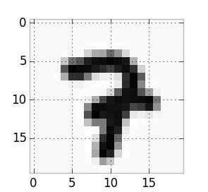
A seven example with a crossed stem
When you train on these examples the model will not generalize well to new examples that do not have this feature. We could say that it would give too much weight to this crossed stem feature. A great measure against over-fitting is having lots and lots of data to train your model on, because the more data you have the less likely you are to have this type of scenario. But beyond getting more data, there are a couple of other ways to minimize this over-fitting problem. The standard way is to use regularization, where you penalize the weights such that minimizing the cost necessarily means shrinking the weights towards 0. Read more about regularization here. However, Hinton et al came up with a solution for neural nets that works by “randomly omitting half of the feature detectors on each training case”. It’s called dropout and it is very effective.
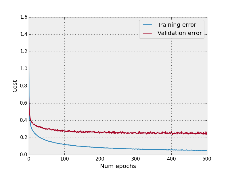
The graph below shows what happens to our validation error, as compared with the training error if we perform no regularization and do not include dropout layers in our model.
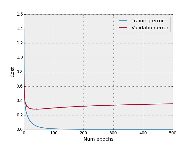
No dropout, no regularization
And here’s what happens with 20% dropout on the input layer and 50% on the hidden layer. Still no regularization.
Dropout layers, no regularization
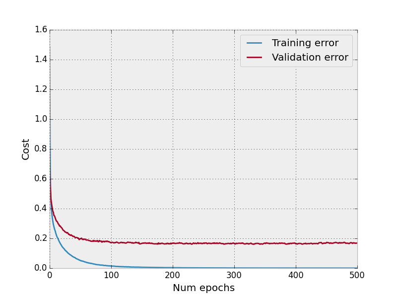
Accuracy on the test set without dropout was generally around 94%, with dropout was around 97%.
If we try without dropout but with l2 regularization it looks like this is not as effective at bringing down the validation error.
Regularization, no dropout
The code for generating the above plots, assuming your training and validation results as returned from lasagne_mlp are in the epoch_cost_train and epoch_cost_val variables respectively, is as follows:
plt.style.use('bmh')
plt.plot(range(len(epoch_cost_train)), epoch_cost_train, label="Training error")
plt.plot(range(len(epoch_cost_val)), epoch_cost_val, label="Validation error")
legend()
plt.xlabel("Num epochs")
plt.ylabel("Cost")
3. Using TensorFlow
In this last section I achieve little more than proving to myself that I can get enough of a handle on things as to be able to adapt the TensorFlow tutorial to my Coursera data set. Go me.
import tensorflow as tf

# This function was copied verbatim from the TensorFlow tutorial at
# https://www.tensorflow.org/versions/master/tutorials/index.html
def dense_to_one_hot(labels_dense, num_classes=10):
  """Convert class labels from scalars to one-hot vectors."""
  num_labels = labels_dense.shape[0]
  index_offset = np.arange(num_labels) * num_classes
  labels_one_hot = np.zeros((num_labels, num_classes))
  labels_one_hot.flat[index_offset + labels_dense.ravel()] = 1
  return labels_one_hot

# Adapted from the TensorFlow tutorial at
# https://www.tensorflow.org/versions/master/tutorials/index.html
class DataSet(object):
  def __init__(self, images, labels):
    assert images.shape[0] == labels.shape[0], (
      "images.shape: %s labels.shape: %s" % (images.shape,
                                             labels.shape))
    self._num_examples = images.shape[0]
    self._images = images
    self._labels = labels
    self._epochs_completed = 0
    self._index_in_epoch = 0
  @property
  def images(self):
    return self._images
  @property
  def labels(self):
    return self._labels
  @property
  def num_examples(self):
    return self._num_examples
  @property
  def epochs_completed(self):
    return self._epochs_completed
  def next_batch(self, batch_size):
    """Return the next `batch_size` examples from this data set."""
    start = self._index_in_epoch
    self._index_in_epoch += batch_size
    if self._index_in_epoch > self._num_examples:
      # Finished epoch
      self._epochs_completed += 1
      # Shuffle the data
      perm = np.arange(self._num_examples)
      np.random.shuffle(perm)
      self._images = self._images[perm]
      self._labels = self._labels[perm]
      # Start next epoch
      start = 0
      self._index_in_epoch = batch_size
      assert batch_size <= self._num_examples
    end = self._index_in_epoch
    return self._images[start:end], self._labels[start:end]
def read_data_sets(train_images, train_labels, validation_images, validation_labels, test_images, test_labels):
  class DataSets(object):
    pass
  data_sets = DataSets()
  data_sets.train = DataSet(train_images, dense_to_one_hot(train_labels))
  data_sets.validation = DataSet(validation_images, dense_to_one_hot(validation_labels))
  data_sets.test = DataSet(test_images, dense_to_one_hot(test_labels))
  return data_sets

# Adapted from the TensorFlow tutorial at
# https://www.tensorflow.org/versions/master/tutorials/index.html
def tensorFlowBasic(X_train, y_train, X_val, y_val, X_test, y_test):
    sess = tf.InteractiveSession()
    x = tf.placeholder("float", shape=[None, 400])
    y_ = tf.placeholder("float", shape=[None, 10])
    W = tf.Variable(tf.zeros([400,10]))
    b = tf.Variable(tf.zeros([10]))
    sess.run(tf.initialize_all_variables())
    y = tf.nn.softmax(tf.matmul(x,W) + b)
    cross_entropy = -tf.reduce_sum(y_*tf.log(y))
    train_step = tf.train.GradientDescentOptimizer(0.01).minimize(cross_entropy)
    mydata = read_data_sets(X_train, y_train, X_val, y_val, X_test, y_test)

    for i in range(1000):
      batch = mydata.train.next_batch(50)
      train_step.run(feed_dict={x: batch[0], y_: batch[1]})

    correct_prediction = tf.equal(tf.argmax(y,1), tf.argmax(y_,1))
    accuracy = tf.reduce_mean(tf.cast(correct_prediction, "float"))
    return accuracy.eval(feed_dict={x: mydata.test.images, y_: mydata.test.labels})

def weight_variable(shape):
  initial = tf.truncated_normal(shape, stddev=0.1)
  return tf.Variable(initial)

def bias_variable(shape):
  initial = tf.constant(0.1, shape=shape)
  return tf.Variable(initial)

def conv2d(x, W):
  return tf.nn.conv2d(x, W, strides=[1, 1, 1, 1], padding='SAME')

def max_pool_2x2(x):
  return tf.nn.max_pool(x, ksize=[1, 2, 2, 1],
                        strides=[1, 2, 2, 1], padding='SAME')

def tensorFlowCNN(X_train, y_train, X_val, y_val, X_test, y_test, add_second_conv_layer = True):
    x = tf.placeholder("float", shape=[None, 400])
    y_ = tf.placeholder("float", shape=[None, 10])
    sess = tf.InteractiveSession()
    # First Convolutional Layer
    W_conv1 = weight_variable([5, 5, 1, 32])
    b_conv1 = bias_variable([32])
    x_image = tf.reshape(x, [-1,20,20,1])
    h_conv1 = tf.nn.relu(conv2d(x_image, W_conv1) + b_conv1)
    h_pool1 = max_pool_2x2(h_conv1)
    if add_second_conv_layer:
        # Second Convolutional Layer
        W_conv2 = weight_variable([5, 5, 32, 64])
        b_conv2 = bias_variable([64])
        h_conv2 = tf.nn.relu(conv2d(h_pool1, W_conv2) + b_conv2)
        h_pool2 = max_pool_2x2(h_conv2)

        # Densely Connected Layer
        W_fc1 = weight_variable([5 * 5 * 64, 1024])
        b_fc1 = bias_variable([1024])
        h_pool2_flat = tf.reshape(h_pool2, [-1, 5*5*64])
        h_fc1 = tf.nn.relu(tf.matmul(h_pool2_flat, W_fc1) + b_fc1)
    else:
        # Densely Connected Layer
        W_fc1 = weight_variable([10 * 10 * 32, 1024])
        b_fc1 = bias_variable([1024])
        h_pool1_flat = tf.reshape(h_pool1, [-1, 10*10*32])
        h_fc1 = tf.nn.relu(tf.matmul(h_pool1_flat, W_fc1) + b_fc1)

    # Dropout
    keep_prob = tf.placeholder("float")
    h_fc1_drop = tf.nn.dropout(h_fc1, keep_prob)
    # Softmax
    W_fc2 = weight_variable([1024, 10])
    b_fc2 = bias_variable([10])
    y_conv=tf.nn.softmax(tf.matmul(h_fc1_drop, W_fc2) + b_fc2)

    # Train the model
    mydata = read_data_sets(X_train, y_train, X_val, y_val, X_test, y_test)
    cross_entropy = -tf.reduce_sum(y_*tf.log(y_conv))
    train_step = tf.train.AdamOptimizer(1e-4).minimize(cross_entropy)
    correct_prediction = tf.equal(tf.argmax(y_conv,1), tf.argmax(y_,1))
    accuracy = tf.reduce_mean(tf.cast(correct_prediction, "float"))
    sess.run(tf.initialize_all_variables())
    for i in range(1000):
        batch = mydata.train.next_batch(50)
        if i%100 == 0:
            train_accuracy = accuracy.eval(feed_dict={
                x:batch[0], y_: batch[1], keep_prob: 1.0})
            print("step %d, training accuracy %g"%(i, train_accuracy))
        train_step.run(feed_dict={x: batch[0], y_: batch[1], keep_prob: 0.5})

    return accuracy.eval(feed_dict={
        x: mydata.test.images, y_: mydata.test.labels, keep_prob: 1.0})
There’s a tensorFlowBasic function which just has an input layer and an output layer, but the fun stuff happens in tensorFlowCNN, which is my first introduction to convolutional neural nets.
accuracy = tensorFlowCNN(X_train, y_train, X_val, y_val, X_test, y_test)
step 0, training accuracy 0.1
step 100, training accuracy 0.82
...
step 900, training accuracy 0.96
accuracy: 0.95200002
I can also pass a parameter telling it not to add a second convolutional layer:
accuracy = tensorFlowCNN(X_train, y_train, X_val, y_val, X_test, y_test, add_second_conv_layer=False)
accuracy: 0.94160002
With the second layer I generally get around 95% accuracy on the test set, without it around 94%. I need to do a lot more experimenting to get a real handle on how to tweak these layers though. And I need to do a lot more reading to understand convolution and pooling better.
Further reading
As mentioned at the start, this exercise has mostly just made me realize how much I have yet to learn about this field. Here’s what I have on my reading list:
- Understanding Convolution in Deep Learning
- Deep Learning in a Nutshell: Core Concepts
- Deep Learning in a Nutshell: History and Training
- Michael Nielson’s Neural Networks and Deep Learning ebook
- Stanford course notes on Convolutional Neural Networks for Visual Recognition
Some TensorFlow-specic stuff: