From both sides now: the math of linear regression

Jun 2, 2016 · 15 minute read · Comments

Linear regression is the most basic and the most widely used technique in machine learning; yet for all its simplicity, studying it can unlock some of the most important concepts in statistics.

If you have a basic undestanding of linear regression expressed as $ \hat{Y} = \theta_0 + \theta_1X$, but don’t have a background in statistics and find statements like “ridge regression is equivalent to the maximum a posteriori (MAP) estimate with a zero-mean Gaussian prior” bewildering, then this post is for you. (And yes, it’s for me as much as it’s for you because I was there not long ago.) With a superficial goal of understanding that somewhat obtuse statement, its main objective is to explore the topic, starting from the standard formulation of linear regression, moving on to the probabilistic approach (maximum likelihood formulation) and from there to Bayesian linear regression.

I’ll use the $\theta$ character throughout to refer to the coefficients (weights) of a regression model, either explicitly broken out as $\theta_0$ and $\theta_1$ for intercept and slope respectively, or just $\theta$ referring to the vector of coefficients. I’ll usually use the expression $\theta^Tx_i$ for the prediction a model gives at $x_i$, the assumption being that a 1 has been added to the vector of values at $x_i$. ¹

What’s in a line?

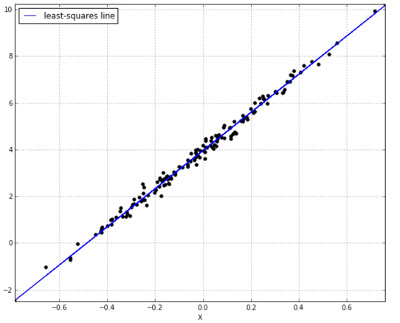
In the single predictor case, we know that the least squares fit is the line that minimizes the sum of the squared distances between observed data and predicted values, i.e. it minimizes the Residual Sum of Squares (RSS):

where is the predicted outcome for the ith observation. We can write the actual value of the ith observation as:

where $\epsilon_i$ is the residual, or error, we get for the ith observation, i.e. the difference between the predicted value $\hat{y_i}$ and the actual value $y_i$.

These residuals are pretty important in how we reason about our model. For now we’ll just note that by definition they must have an expected value (mean) of 0.

What else can we say about this line? It defines a particular relationship between the predictor and the outcome. Specifically, the slope of the line is the correlation between outcome values and predictor values, multiplied by the ratio of their standard deviations. So we know how to calculate $\theta_1$ from our data. What about $\theta_0$? Well, we know that the line goes through the point (mean(x), mean(y))², and once we know the slope of a line and a single point it goes through we can find the intercept by working back along the slope from that point: $\theta_0 = \bar{y} - \theta_1\bar{x}$

In the multiple regression scenario, where we have p predictors, we model the outcome as:

$ \hat{y_i} = \theta_0 + \theta_1x_1 + \theta_2x_2 + … + \theta_px_p $

In this setting it’s not quite as straight-forward to derive the coefficients as in the single predictor case. Instead, we need to use calculus and get the partial derivative of our cost function with respect to each parameter and solve for that parameter when setting its derivative to 0.³

From minimization to maximization

If we ever want to understand linear regression from a Bayesian perspective we need to start thinking probabilistically. We need to flip things over and instead of thinking about the line minimizing a cost, think about it as maximizing the likelihood of the observed data. As we’ll see, this amounts to the exact same thing - mathematically speaking - it’s just a different way of looking at it.

To get the likelihood of our data given our assumptions about how it was generated, we must get the probability of each data point y and multiply them together.

We want to find values of $\theta$ that maximize this result.

How do we calculate each of these probabilities?

Know thy Normal distribution

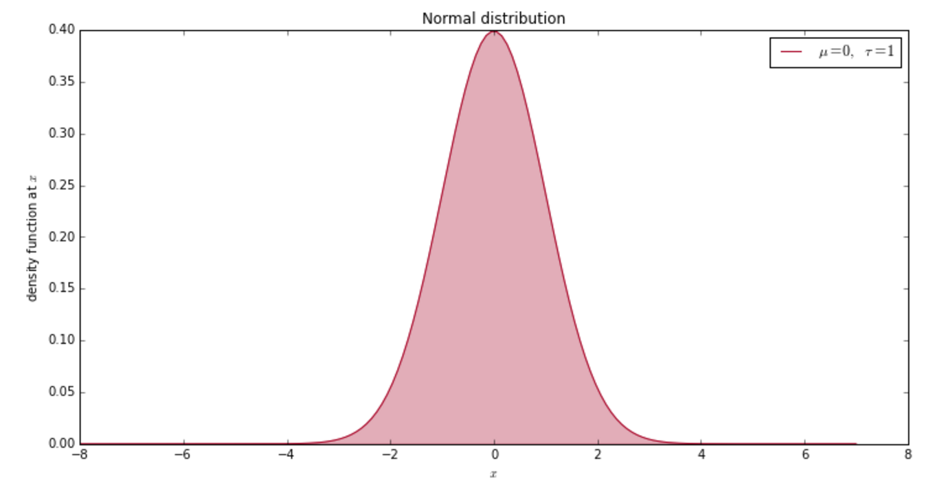
We noted earlier that the residuals from our least squares fit have a mean of 0. Well we can go one step and say that they are normally distributed with a mean of 0, i.e.

Here’s the function that defines the normal, or Gaussian, distribution: It’s not the friendliest looking function, but there’s really no way around it: you have to learn this function off because you’ll need to be able to recognize it when you see it in equations. A handy fact about the normal distribution is that if $ X \sim \mathcal{N}(\mu, \sigma^2)$ and $Y \sim \mathcal{N}(0, \sigma^2)$ then $ X = \mu + Y$⁴

Back to calculating the probabilities of our observed y values… if each $y_i$ is $\theta^Tx_i + \epsilon_i$ and $\epsilon_i \sim \mathcal{N}(0, \sigma^2)$, we can also say that

See what we did there? We used our handy fact about normally distributed variables, only in reverse. And now we have a way of calculating the probability of each $y_i$ - we just plug it into the normal density function with the right mean and variance. Here’s a python function that will calculate the log-likelihood of our y values given the x values and a model as specified by theta0, theta1 and standard deviation.

def log_likelihood(x, y, theta0, theta1, stdev):
    # Get the likelihood of y given the least squares model described
    # by theta0, theta1 and the standard deviation of the error term.
    for i, x_val in enumerate(x):
        mu = theta0 + (theta1*x_val)
        # This is just plugging our observed y value into the normal
        # density function.
        lk = stats.norm(mu, stdev).pdf(y[i])
        res = lk if i == 0 else lk * res
    return Decimal(res).ln()

We often work with the log-likelihood instead of the likelihood simply because it produces quanitities that are easier to work with and compare. And because the log function is a monotonically increasing function, we know that maximizing the log of a value, with respect to some parameter, coincides with maximizing the value itself.

We want to maximize the likelihood of our data with respect to our parameters, $\theta$. Here’s that likelihood shown as the product of normal densities:

With a little mathematical shunting (and remembering that $e^xe^y = e^{x + y}$) we can see that this is equivalent to: Anything look familiar there? Yay - it’s our RSS! Hopefully you can see that minimizing the highlighted part of this expression means maximizing the entire expression. In other words, minimizing the residual sum of squares is equivalent to maximizing the likelihood of the data.

And to get a visual feel for this likelihood, here’s a contour plot:

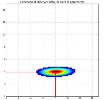
This was produced based on the same data I generated for the linear regression line above. I plugged the Xs and Ys and a series of possible $(\theta_0,\theta_1)$ pairs into the log_likelihood function above to get the log-likelihood of each combination. The original data were generated with an intercept of 4 and a slope of 8 (i.e. y = 4 + 8x + noise.)

Bayesian Inference

Now that we’re thinking in terms of likelihood of data, we can start to adopt a Bayesian mindset.

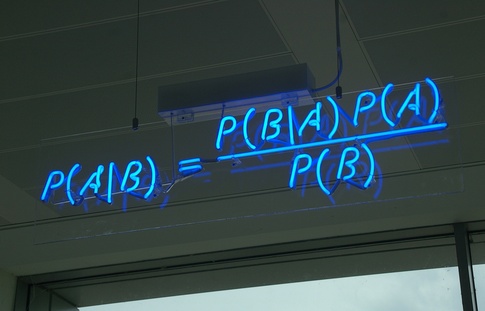
Source: Wikipedia

Hopefully you have come across Bayes’ Rule before - it describes the conditional probability of event A given event B. A note on the bottom line on the right hand side: you may have seen the rule written as

But because that bottom line exhausts all possibilities with respect to event A, it boils down to simply p(B). So event A has been “marginalized out”. (In the discrete case you’re talking about probabilities over the possible values of A, which you could tabulate, summing the totals in the margins, hence marginalized.) So this quantity is referred to as the “marginal likelihood”, and because it isn’t dependent on event A, it is often removed from the equation and the rule is expressed as a proportion instead: The way Bayes rule is used for Bayesian inference is that your model is conditioned on your data: where H stands for hypothesis and D stands for data. Sometimes you’ll see the word evidence used in place of data. And with this interpretation of the rule, we can now finally talk about priors and posteriors. In the Bayesian setting, the term probability is used as a measure of belief in a hypothesis. You start with a prior belief about that hypothesis, then observe some data (or “gather evidence”), and then you have a posterior belief.

or

One other really important thing to note about Bayesian methods is that they are always explicit about uncertainty. They work with probability distritions, not point estimates. So a hypothesis about the parameters of a linear model would not be e.g. that the intercept has a value of 4, but that it is normally distributed with a mean of 4 and some standard deviation. And this gets updated the more evidence you gather. So your prior is a distribution and so is your posterior.

The way I like to think of it is that the data is like a magnet that attracts probability mass.

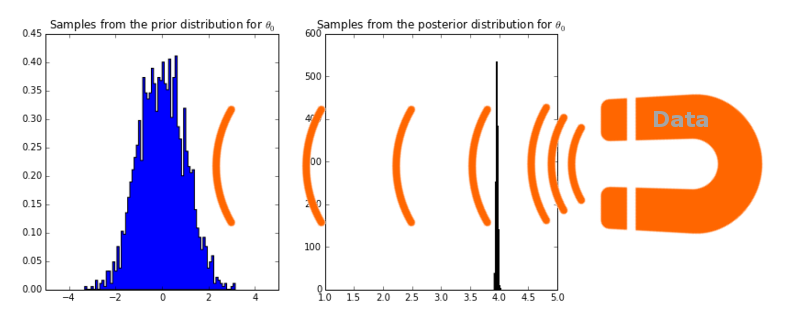
On the left you see samples from the prior distribution I gave for the intercept parameter, $\theta_0$: normally distruted with mean 0 and standard deviation 1. I then used PyMC, a Python module for doing Markov Chain Monte Carlo sampling, to come up with the posterior distribution on the right. The mean (and the mode) of this posterior distribution is 3.95, close to the true parameter of 4. This is our maximum a posteriori (MAP) estimate for the $\theta_0$ parameter.

But before we continue on our journey to understand what MAP estimates have to do with ridge regression, we must finish our exploration of regression in the Bayesian setting. It’s interesting to see what happens if instead of using a prior that’s normally distributed with mean 0 and standard deviation of 1, we give it a uniform prior between -2 and 2.

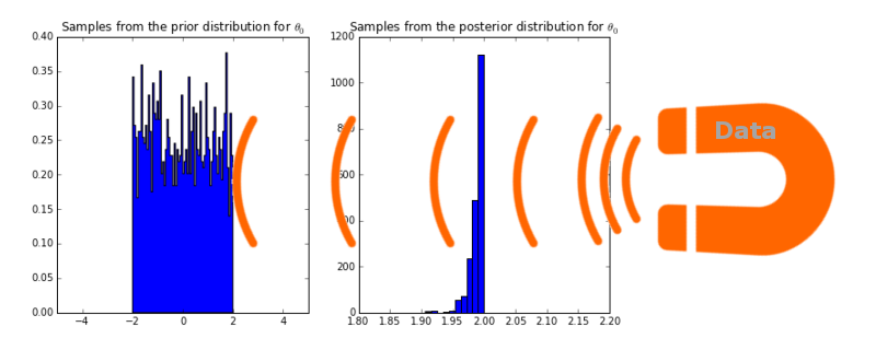
No matter how strong that magnet, i.e. no matter how much data we gather, the posterior will never assign a non-zero probability to any value greater than 2. So obviously it’s important to choose a sensible prior.

Once we have a posterior for each parameter, one way we could go about making predictions would be to simply “plug in” the MAP estimates of our parameters:

$\hat{y^*} = [\text{MAP estimate of }\theta_0] + [\text{MAP estimate of }\theta_1] x^* $

where $ x^* $ is an unseen data point for which we want to predict the outcome $ y^* $. That is frequentist thinking though. Remember, Bayesians work with distributions, not point estimates, and so no special significance is bestowed upon MAP estimates in the Bayesian setting. The way prediction works instead is that we get a probability distribution (of course!) for the outcome $ y^* $ at each $ x^* $. We use the posterior distribution of the weights, representing all possible linear models, each of which would produce a different prediction for y. And so the prediction from each possible model is weighted by the probability of that model. Or, more formally:

$ p(y^* | x^*, X, y) = \int_{\theta}p(y^* | x^*,\theta)p(\theta|X,y)d\theta $

X and y are given - they are the training data; $ x^* $ is also given - it’s the new data point we want to predict the outcome for. From those three givens we want to predict $ y^* $. And we do it by marginalizing (remember that term?) over the posterior distribution of $\theta$. What we end up with is a Gaussian distribution whose variance depends on the magnitude of the $ x^* $ value.

The beauty of this is that it retains information about the level of uncertainty around each prediction.

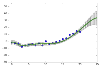
The further away we get from our training data, the greater the margin of error around our predictions.

It’s always seemed obvious to me that it’s better to know that you don’t know, than to think you know and act on wrong information. But it surprised me to learn years ago that there are people who prefer to have “an answer” they can act upon and aren’t too concerned about whether it’s correct. They may be the same people who will tell me something with great confidence when they have absolutely no idea what they’re talking about. Personally, I’ve always preferred interacting with the “wiser people so full of doubts”. I guess that makes me a Bayesian.

Anyway, back to statistics.

MAP estimates and Ridge Regression

It’s finally time to make sense of that statement about the relationship between ridge regression and MAP estimates. Ridge regression is about penalizing large values of parameters in order to prevent over-fitting to your training data. Here’s an example from Kevin Murphy’s companion code to his textbook on machine learning. We have generated some dummy data where the true function that produces y from x is a second-order polynomial function ($ y = ax + bx^2 $.) But we are trying to fit a 14-degree polynomial to the data.

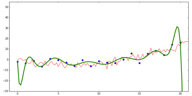
The green line represents predictions for the test set based on the weights learned for the training set. The red line represents the true values of the test set. We can see that the green line fits the training values very well, but it does this by being very “loopy” - due to some weights having extremely high positive values and others having extreme negative values. This makes it go wildly wrong on some of the test data. If we penalize extreme values, this forces the model to fit the data in a way that’s more likely to generalize to unseen data. With ridge regression, we do this by adding the sum of the squared parameters to the cost that we’re minimizing:

where $ \lambda $ is a tuning parameter that controls the extent to which the weights are penalized and p is the length of the parameter vector $\theta$, excluding the intercept. For a really great explanation of ridge regression, I highly recommend the Hastie et al book An Introduction to Statistical Learning.

Now let’s see how we can arrive at this same solution from the Bayesian method. Recall that the posterior distribution for the weights is proportional to the likelihood times the prior. Using the likelihood we figured out before and a Gaussian prior with a mean of 0 and a variance of $\tau^2$, this becomes:

with the likelihood in blue and the prior in green. With some slight rearranging we get

Given that we are looking to maximize this with respect to the coefficients, we can ignore the terms that don’t depend on the coefficients:

And remember that we like to work with the log-likelihood instead of the likelihood, so now we have

Multiplying by $2\sigma^2$ and pulling out the -1 we get:

And since maximizing $-x$ is equivalent to minimizing $x$, this is equivalent to:

And this is exactly what we have above for a regularized cost function, only with $ \frac{\sigma^2}{\tau^2} $ instead of $ \lambda $.

So we have shown that ridge regression is indeed equivalent to a maximum a posteriori estimate with a zero-mean Gaussian prior, with $\lambda$ proportional to $\tau^2$. Specifically, a lower variance on the prior for the weights (i.e. a more constrained prior) is equivalent to a higher $\lambda$ value in the ridge regression solution.

Q.E.D. :)

In conclusion

We’ve looked at linear regression from both sides now - from the frequentist and Bayesian perspectives, and still somehow…

No no no, this isn’t going to end like the song - I think we know linear regression fairly well after all that. However, there’s always more to learn and so I’ll leave you with some of the resources I’ve found to be most helpful in understanding this stuff.

Further Reading

If you don’t yet have a copy of An Introduction to Statistical Learning by James, Witten, Hastie and Tibshirani, what are you waiting for? The whole thing is available as a freely downloadable PDF and provides the most crystal clear explanation of linear regression and regularization I’ve ever come across. Another freely downloadable book is Gaussian Processes for Machine Learning by Rasmussen and Williams. I think this may have been the first place I was introduced to the relationship between MAP estimates and ridge regression. Kevin Murphy’s Machine Learning - a Probabilistic Approach provides a very complete explanation of this and a whole lot more - it is a pretty enormous tome, and while I do aspire to reading the whole thing… well, it’ll take some time ;)

And finally, while reading textbooks is totally awesome and worthwhile and in fact my favourite way to get a handle on topics like this, nothing beats playing around with code to get a more complete understanding of the ideas. Cameron Davidson-Pilon’s Probabilistic Programming & Bayesian Methods for Hackers is a fantastic introduction to Markov Chain Monte Carlo and the PyMC Python library. And it’s also available for free online!